

Lead Time to Change #
Part of the Dora Metrics documentation. For the metric cards, the graph types, the Application Metric Table and service-level metrics, see the Dora Metrics Guide. For how to open the dashboard and choose a date range, see the Maturity Insights Overview.
What is Lead Time to Change? #
Lead Time to Change (LTTC) measures the average time taken for code changes to move from the initial commit to a successful production deployment. For each deployment, BuildPiper identifies all merged pull requests between the current and previous deployments’ commits, and calculates the time from each pull request’s initial commit to the deployment time. The average of these durations is recorded as that deployment’s LTTC.
LTTC helps measure delivery efficiency by showing how quickly code changes reach production. A lower LTTC typically indicates faster feedback cycles, improved engineering productivity and a more responsive software delivery process. A lower value is better.
To view it, select the Lead Time to Change card on the Dora Metrics dashboard. The graphs below the cards then show its trend, thresholds, maturity levels, top performing applications, applications that need attention and benchmarks. This guide explains how the metric is calculated and how to read each graph.
How Lead Time to Change is calculated #
You can also see this explanation on the dashboard: click How it Works in the Thresholds Legend.
Lead Time to Change is measured as a time value. It uses the Per Scan aggregation (each deployment’s LTTC is one record, and the records are averaged) and the Highest rating rule.
What is counted #
For each successful production deployment, BuildPiper looks at the pull requests merged between the previous deployment and the current one, and calculates how long those changes took to reach production.
How the value is calculated #
- 1
For each successful production deployment, BuildPiper finds every pull request merged between the previous deployment and this one.
- 2
It calculates the time from the pull request’s first associated commit to the deployment completion time.
- 3
It averages these times across all the merged pull requests in that deployment.
- 4
It averages the LTTC values of all deployments in the selected date range. This is the value shown on the dashboard.
Formula #
| Value | Formula |
|---|---|
| Lead time for a pull request | Production deployment time − First associated commit time |
| LTTC for a deployment | Sum of lead times for all merged pull requests in the deployment ÷ Number of merged pull requests |
| Overall LTTC | Sum of deployment LTTC values ÷ Number of deployments |
Worked example #
A deployment includes 3 pull requests merged since the previous deployment:
| Pull request | Lead time |
|---|---|
| PR-101 | 128 hours |
| PR-102 | 76 hours |
| PR-103 | 33 hours |
The LTTC for this deployment is (128 + 76 + 33) ÷ 3 = 79 hours.
If a service has three deployments in the selected period, with LTTC values of 79, 50 and 60 hours, the LTTC shown for the period is (79 + 50 + 60) ÷ 3 = 63 hours.
At service, application and organization level #
The LTTC at each level is the average of all deployment-level LTTC values within it:
| Level | Calculation | LTTC shown |
|---|---|---|
| Service with 3 deployments | (79 + 50 + 60) ÷ 3 | 63 hours |
| Application with 5 deployments across its services | (79 + 50 + 60 + 40 + 30) ÷ 5 | 51.8 hours |
| Organization with 7 deployments across all applications | (79 + 50 + 60 + 40 + 30 + 24 + 36) ÷ 7 | 45.57 hours |
Good to know: Unlike Deployment Frequency, LTTC is an average, so it does not grow with the number of services. An application or organization with many fast deployments can have a lower LTTC than some of its individual services.
Lead Time to Change graphs #
Each graph type is introduced in “Metric graphs” in the Dora Metrics Guide. This section shows what each graph looks like for Lead Time to Change and how to read it.
Lead Time to Change Trend #
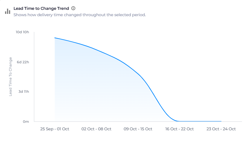
What it shows: How delivery time changed during the selected period. It highlights faster delivery periods, delays, spikes and recurring patterns in the time it takes changes to reach production.
Example: Lead time was about 9 days in the week of 25 September–1 October and fell steadily over the following weeks, reaching 0m from 16 October onward.
Use it to: See whether changes are reaching production faster or slower over time, and spot delays.
Thresholds Legend #
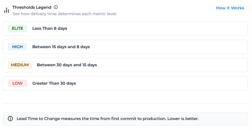
What it shows: The time thresholds that assign each level. Lower values represent faster delivery.
| Level | Lead Time to Change |
|---|---|
| Elite | Less than 8 days |
| High | Between 8 and 15 days |
| Medium | Between 15 and 30 days |
| Low | More than 30 days |
Unlike Deployment Frequency, these thresholds are fixed times. They do not change with the length of the selected period or the number of services.
Use it to: Know how much faster changes need to reach production to move up a level.
Metal Rating Distribution #

What it shows: How applications are spread across the Lead Time to Change levels.
Example: 4 applications are Elite and 3 are High. None are Medium or Low, so every application gets changes to production in under 15 days.
Use it to: Understand how delivery speed is spread across your applications.
Applications Top Performing #

What it shows: The applications that took the least time to move code changes into production.
Example: PMS, ToolHub, KubeLift and SentryFuse have a lead time close to zero, while SpendSmart takes a little over 8 days.
Use it to: Identify the fastest-delivering applications and learn from their practices.
Need Attention Applications #
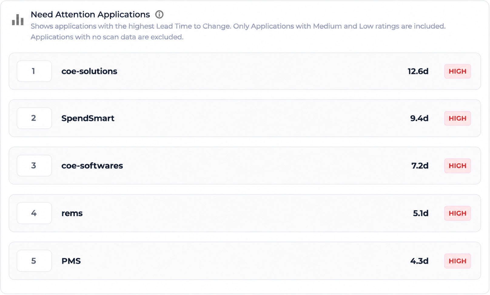
What it shows: The applications that took the most time to move code changes into production, ranked from slowest to fastest, with their lead time and level.
Example: coe-solutions has the longest lead time at 12.6 days, followed by SpendSmart (9.4 days), coe-softwares (7.2 days), rems (5.1 days) and PMS (4.3 days).
Use it to: Find the applications where changes take longest to reach production, and focus improvement efforts there first.
Lead Time to Change Benchmarks #
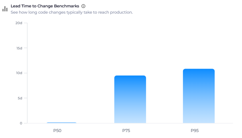
What it shows: How long code changes typically take to reach production, using percentiles:
| Percentile | Meaning |
|---|---|
| P50 | The median Lead Time to Change: half of changes reach production in this time or less. |
| P75 | 75% of changes reach production in this time or less. |
| P95 | 95% of changes reach production in this time or less. P75 and P95 show the higher end of the delivery-time distribution. |
Example: P50 is close to zero, but P75 is about 9.5 days and P95 is about 11 days. Most changes reach production almost immediately, but a quarter of them take more than 9 days.
Use it to: See what typical delivery time looks like, and how far the slowest changes are from it.